When you’re on your computer and want to crunch some numbers, you use a program called a spreadsheet. There are several different spreadsheet programs available for your personal computer.

Full-featured spreadsheet programs include Microsoft Excel, Lotus 1-2-3, and Corel’s Quattro Pro; for more casual users, there’s also the Works Spreadsheet included in Microsoft Works and Works Suite.

The most popular spreadsheet among serious number crunchers is Microsoft Excel, which is included as part of the Microsoft Office suite. That’s the spreadsheet we’ll look at in this tutorial, although the other spreadsheet programs operate in a similar fashion.

What is Spreadsheets?

A spreadsheet is nothing more than a giant list. Your list can contain just about any type of data you can think of—text, numbers, and even dates. You can take any of the numbers on your list and use them to calculate new numbers. You can sort the items on your list, pretty them up, and print the important points in a report.

You can even graph your numbers in a pie, line, or bar chart! All spreadsheet programs work in pretty much the same fashion. In a spreadsheet, everything is stored in little boxes called cells. Your spreadsheet is divided into lots of these cells, each located in a specific location on a giant grid made of rows and columns.

Each single cell represents the intersection of a particular row and column. As you can see in Figure 1, each column has an alphabetic label (A, B, C, and so on). Each row, on the other hand, has a numeric label (1, 2, 3, and so on).

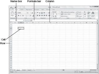
The location of each cell is the combination of its column and row locations. For example, the cell in the upper-left corner of the spreadsheet is in column A and row 1; therefore, its location is signified as A1. The cell to the right of it is B1, and the cell below A1 is A2.

The location of the selected, or active, cell is displayed in the Name box. Next to the Name box is the Formula bar, which echoes the contents of the active cell. You can type data directly into either the Formula bar or active cell.

Entering Data

Entering text or numbers into a spreadsheet is easy. Just remember that data is entered into each cell individually—then you can fill up a spreadsheet with hundreds or thousands of cells filled with their own individual data. To enter data into a specific cell, follow these steps:

1. Select the cell you want to enter data into.
2. Type your text or numbers into the cell; what you type will be echoed in the Formula bar at the top of the screen.
3. When you’re done typing data into the cell, press Enter.

Inserting and Deleting Rows and Columns

Sometimes you need to go back to an existing spreadsheet and insert some new information.

Insert a Row or Column

To insert a new row or column in the middle of your spreadsheet, follow these steps:

1. Click the row or column header after where you want to make the insertion.
2. In Excel 2007, go to the Cells section of the Ribbon and click the down arrow next to the Insert button; then select either Insert Sheet Rows or Insert Sheet Columns. In Excel 2003, pull down the Insert menu and select either Insert Row or Insert Column.

Excel now inserts a new row or column either above or to the left of the row or column you selected.

Delete a Row or Column

To delete an existing row or column, follow these steps:

1. Click the header for the row or column you want to delete.
2. In Excel 2007, go to the Cells section of the Ribbon and click the Delete button. In Excel 2003, pull down the Edit menu and select Delete.

The row or column you selected is deleted, and all other rows or columns move up or over to fill the space.

Adjusting Column Width

If the data you enter into a cell is too long, you’ll only see the first part of that data—there’ll be a bit to the right that looks cut off. It’s not cut off, of course; it just can’t be seen, since it’s longer than the current column is wide. You can fix this problem by adjusting the column width.

Wider columns allow more data to be shown; narrow columns let you display more columns per page. To change the column width, move your cursor to the column header, and position it on the dividing line on the right side of the column you want to adjust.

When the cursor changes shape, click the left button on your mouse and drag the column divider to the right (to make a wider column) or to the left (to make a smaller column). Release the mouse button when the column is the desired width.

Using Formulas and Functions

Excel lets you enter just about any type of algebraic formula into any cell. You can use these formulas to add, subtract, multiply, divide, and perform any nested combination of those operations.

Creating a Formula

Excel knows that you’re entering a formula when you type an equal sign (=) into any cell. You start your formula with the equal sign and enter your operations after the equal sign.

For example, if you want to add 1 plus 2, enter this formula in a cell: =1+2. When you press Enter, the formula disappears from the cell—and the result, or value, is displayed.

Including Other Cells in a Formula

If all you’re doing is adding and subtracting numbers, you might as well use a calculator. Where a spreadsheet becomes truly useful is when you use it to perform operations based on the contents of specific cells. To perform calculations using values from cells in your spreadsheet, you enter the cell location into the formula.

For example, if you want to add cells A1 and A2, enter this formula: =A1+A2. And if the numbers in either cell A1 or A2 change, the total will automatically change, as well. An even easier way to perform operations involving spreadsheet cells is to select them with your mouse while you’re entering the formula.

To do this, follow these steps:

1. Select the cell that will contain the formula.
2. Type =.
3. Click the first cell you want to include in your formula; that cell location is automatically entered in your formula.
4. Type an algebraic operator, such as +, -, *, or /.
5. Click the second cell you want to include in your formula.
6. Repeat steps 4 and 5 to include other cells in your formula.
7. Press Enter when your formula is complete.

Quick Addition with AutoSum

The most common operation in any spreadsheet is the addition of a group of numbers. Excel makes summing up a row or column of numbers easy via the AutoSum function. All you have to do is follow these steps:

1. Select the cell at the end of a row or column of numbers, where you want the total to appear.
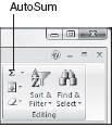
2. Click the AutoSum button in the Editing section of the Ribbon (Excel 2007), as shown in Figure 2, or on the Standard toolbar (Excel 2003).

Other AutoSum Operations

Excel’s AutoSum also includes a few other automatic calculations. When you click the down arrow on the side of the AutoSum button, you can perform the following operations:

• Average, which calculates the average of the selected cells.
• Count Numbers, which counts the number of selected cells.
• Max, which returns the largest value in the selected cells.
• Min, which returns the smallest value in the selected cells.

Using Functions

In addition to the basic algebraic operators previously discussed, Excel also includes a variety of functions that replace the complex steps present in many formulas. For example, if you wanted to total all the cells in column A, you could enter the formula =A1+A2+A3+A4.

Or, you could use the SUM function, which lets you sum a column or row of numbers without having to type every cell into the formula. (And when you use AutoSum, it’s simply applying the SUM function.) In short, a function is a type of prebuilt formula.

You enter a function in the following format: =function(argument), where function is the name of the function and argument is the range of cells or other data you want to calculate. Using the last example, to sum cells A1 through A4, you’d use the following function-based formula: =sum(A1,A2,A3,A4). Excel includes hundreds of functions.

You can access and insert any of Excel’s functions by following these steps:

1. Select the cell where you want to insert the function.
2. In Excel 2007, select the Formulas Ribbon
3. From here you can click a function category to see all the functions of a particular type, or click the Insert Function button to display the Function dialog box. Select the function you want.
4. If the function has related arguments, a Function Arguments dialog box is now displayed; enter the arguments and click OK.
5. The function you selected is now inserted into the current cell. You can now manually enter the cells or numbers into the function’s argument.

Sorting a Range of Cells

If you have a list of either text or numbers, you might want to reorder the list for a different purpose. Excel lets you sort your data by any column, in either ascending or descending order. To sort a range of cells, follow these steps:

1. Select all the cells you want to sort.
2. In Excel 2007, click the Sort & Filter button in the Ribbon; then select how you want to sort—A to Z, Z to A, or in a custom order (Custom Sort).
3. If you select Custom Sort, you’ll see the Sort dialog box.
4. From here you can select various levels of sorting; select which column to sort by, and the order from which to sort. Click the Add Level button to sort on additional columns.

Formatting Your Spreadsheet

You don’t have to settle for boring-looking spreadsheets. You can format how the data appears in your spreadsheet—including the format of any numbers you enter.

Applying Number Formats

When you enter a number into a cell, Excel applies what it calls a “general” format to the number—it just displays the number, right-aligned, with no commas or dollar signs. You can, however, select a specific number format to apply to any cells in your spreadsheet that contain numbers.

In Excel 2007, all the number formatting options are in the Number section of the Ribbon. Click the dollar sign button to choose an accounting format, the percent button to choose a percentage format, the comma button to choose a comma format, or the General button to choose from all available formats. You can also click the Increase Decimal and Decrease Decimal buttons to move the decimal point left or right.

Formatting Cell Contents

You can also apply a variety of other formatting options to the contents of your cells. You can make your text bold or italic, change the font type or size, or even add shading or borders to selected cells.

In Excel 2007, these formatting options are found in the Font and Alignment sections of the Ribbon. Just select the cell(s) you want to format; then click the appropriate formatting button.

Creating a Chart

Numbers are fine, but sometimes the story behind the numbers can be better told through a picture. The way you take a picture of numbers is with a chart, such as the one shown in Figure below.

You create a chart based on numbers you’ve previously entered into your Excel spreadsheet. In Excel 2007, it works like this:

1. Select the range of cells you want to include in your chart. (If the range has a header row or column, include that row or column when selecting the cells.)
2. Select the Insert Ribbon.
3. In the Charts section of the Ribbon, click the button for the type of chart you want to create.
4. Excel now displays a variety of charts within that general category. Select the type of chart you want.
5. When the chart appears in your worksheet, select the Design Ribbon to edit the chart’s type, layout, and style; or select the Layout Ribbon to edit the chart’s labels, axes, and background.

In Excel 2003, the process is subtly different. After you select the range of cells, click the Chart Wizard button on the Excel toolbar. This wizard walks you through a series of steps that help you choose the type of chart you want and the formatting for that chart.